Using Analytical Formulas for High-Speed Interconnects: Sources, Validity and Considerations
Essay · Analytical formulas let an engineer size a trace, a via or a channel in seconds. This essay sets out the standard formulas for high-speed interconnects, where each comes from, when it holds, and six considerations that decide whether its answer can be trusted.
Abstract
Field solvers are accurate but slow; analytical formulas are fast but approximate. Most interconnect decisions are made in the fast regime, at the whiteboard, in a spreadsheet or in a design tool that must answer as fast as the user types.
The standard formulas are well established: Hammerstad–Jensen and IPC-2141 for microstrip [1, 3, 4], Cohn's result for stripline [5], conformal mapping for coplanar waveguide [11, 12], Bogatin's loss rules of thumb [7], Johnson and Graham's via estimates [8] and Rosa's wire inductance [18]. Each is valid only over a stated range.
We collect these formulas with their sources and worked examples, then draw out six considerations. The largest effect we found is that a simplified empirical fit for grounded coplanar waveguide reads 14–28% low against conformal mapping, enough to turn a "50 Ω" line into a 70 Ω one.
1. Why analytical formulas
An analytical formula returns in microseconds, where a 2D field solver takes seconds and a 3D solver minutes to hours. That speed makes sweeps, optimisation and interactive design practical. It also makes trends visible: a formula shows at a glance that impedance falls with the logarithm of width, or that dielectric loss rises linearly with frequency.
The price is accuracy. Each formula is either a closed-form solution of an idealised geometry or a curve fitted to solver or measured data. Both hold only inside the conditions under which they were derived or fitted, and both ignore effects their authors set aside.
Lengths below are in mil (1 mil = 25.4 µm), frequencies in GHz and impedances in Ω unless stated.
2. Microstrip
2.1 Thickness correction
Copper thickness T follows from copper weight at about 1.37 mil per ounce. A thick strip behaves like a slightly wider strip of zero thickness. Wheeler's correction [2], in the form Hammerstad and Jensen adopted [1], is:
For W = 8, H = 10 and T = 1.37 this gives Weff = 10.34 mil and u = 1.03.
2.2 Effective permittivity
Part of a microstrip's field runs in air, so the signal sees a permittivity between 1 and Er:
This is the simplified quasi-static form. Hammerstad's full expression adds a term 0.04(1 − u)² for narrow strips with u < 1 [3]. With Er = 3.66 the example gives εeff = 2.70.
2.3 Hammerstad's impedance formulas
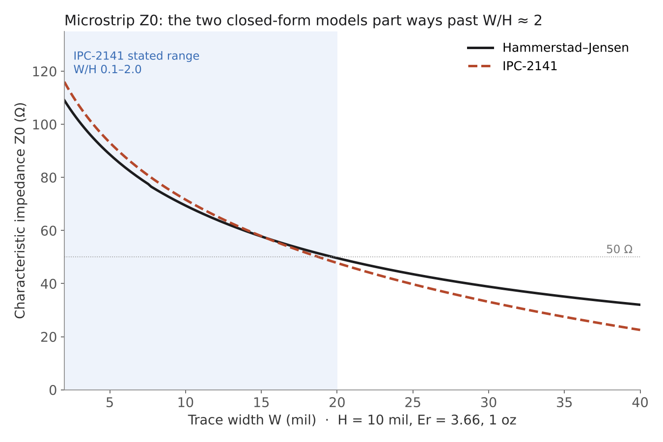
These two-branch formulas are accurate to about 1% [3]. The example gives Z0 = 75.6 Ω; reaching 50 Ω needs W ≈ 19.7 mil, about twice H. Hammerstad and Jensen's 1980 paper replaces the two branches with one expression accurate to 0.01% for u ≤ 1 and 0.03% for u ≤ 1000 [1], which also removes the small step the branches leave at u = 1.
2.4 The IPC-2141 formula
The formula most PCB designers know is the IPC-2141 one [4], which goes back to Kaupp [6]:
It is simpler but stated only for 0.1 < W/H < 2.0 [4]. For the example it gives 78.9 Ω, 4% above Hammerstad, and reaches 50 Ω at W = 18.8 mil.
3. Stripline
A symmetric stripline between planes spaced b apart has Cohn's exact solution [5], usually used in its IPC-2141 approximation [4]:
For W = 6, b = 16, T = 1.37 and Er = 3.66 it gives 50.0 Ω. The range commonly quoted is W/(b − T) < 0.35 and T/b < 0.25. When the trace sits off-centre, IPC-2141 gives a dedicated asymmetric-stripline formula [4]; averaging two symmetric results is a common shortcut with no published basis.
4. Grounded coplanar waveguide
Coplanar waveguide with a lower ground plane is the usual choice above about 20 GHz. Its standard analytical model comes from conformal mapping: Wen for coplanar waveguide [11] and Ghione and Naldi for the grounded version [12], both collected by Wadell [10]:
K is the complete elliptic integral of the first kind and k′ = √(1 − k²). K needs only a few lines of code via the arithmetic–geometric mean. For w = 8, s = 5, h = 8 and Er = 3.38 these give 71.4 Ω and εeff = 2.37.
5. Propagation delay
85 ps/in is the time light takes to cross an inch of vacuum, the inverse of 11.8 in/ns [7]. Stripline uses εeff = Er because its field lies entirely in the dielectric. The microstrip example gives 140 ps/in; stripline at Er = 3.66 gives 163 ps/in.
6. Loss
6.1 Dielectric loss
This is Bogatin's rule of thumb [7]. It is the textbook attenuation π·f·√εr·tanδ/c converted to dB per inch: 8.686 × π / 11.8 = 2.31 [9]. For microstrip, εeff belongs in place of εr. Example: FR-4 with Df = 0.02 and Er = 4.3 loses 0.48 dB/in at 5 GHz.
6.2 Conductor loss
Bogatin's skin-effect rule of thumb [7] captures the two trends that matter: conductor loss rises with √f and falls with width. Kr is a roughness factor. For W = 8 mil and Z0 = 75.6 Ω at 10 GHz on smooth copper it gives 0.188 dB/in.
6.3 Copper roughness
Rough copper lengthens the current path once the skin depth approaches the roughness. Hammerstad and Jensen's correction [1] saturates at 2:
For 1 µm rms roughness it gives 1.20 at 1 GHz and 1.81 at 10 GHz. Huray's snowball model [14] can exceed 2 and fits modern foils better at high frequency.
6.4 Er and Df versus frequency
Laminate datasheets give Er and Df at a few frequencies. Interpolating linearly in log f matches the Djordjevic–Sarkar wideband Debye model, in which Er falls linearly with log f [15]:
Values extrapolated far above the highest datasheet frequency should be confirmed with the fabricator.
7. Vias, wire bonds and connectors
7.1 Signal via
These are Johnson and Graham's equations 7.9 and 7.6 [8], and Johnson calls both crude. The capacitance assumes a solid coaxial ground wall at the anti-pad diameter [16]. The "+1" inductance matches a return path about 5.4h away; the low-frequency partial-inductance form uses −0.75 instead [17].
A via stub resonates at a quarter wavelength:
For a 32 mil board, 8 mil drill, 20 and 30 mil pad and anti-pad and Er = 3.66 these give L = 0.61 nH, C = 0.33 pF, an impedance √(L/C) of 43 Ω and a full-length stub resonance at 48 GHz.
7.2 Wire bond
This is Rosa's partial self-inductance of a straight round wire [18], as tabulated by Grover [19]. At high frequency, where skin effect removes the internal inductance, the constant becomes −1 [17]. Parallel bonds do not divide inductance by their count, because their mutual inductance adds back.
Treating the bond as a series reactance X between ports of impedance Z0 gives |S21|² = 1/[1 + (X/2Z0)²] [9]. A 40 mil gold bond of 1 mil diameter has about 0.9 nH, 55 Ω of reactance at 10 GHz and 1.2 dB of loss in a 50 Ω system.
7.3 Coaxial connectors
Each precision series is rated to its mode-free limit: 2.92 mm to 40 GHz, 2.4 mm to 50 GHz and 1.85 mm to 67 GHz [21]; SMA is commonly rated to 18 GHz. Below those limits, connector loss and match depend on the launch design more than on any formula.
8. Reflections and mismatch
These are exact definitions [9]. A 45 Ω via on a 50 Ω line gives 25.6 dB return loss and 0.012 dB mismatch loss.
9. Channel-level models
9.1 Nyquist and knee frequency
The 0.35/tr relation is the single-pole bandwidth of a rising edge [8]. A 35 ps edge has a 10 GHz knee.
9.2 S-parameters of a lossy line
This is the standard ABCD description of a transmission line [9]. α comes from section 6, converted from dB to nepers by dividing by 8.686, and launch parasitics cascade as further ABCD matrices.
9.3 Crosstalk and eye
Near-end crosstalk between parallel traces over a plane falls roughly as 1/[1 + (s/h)²] with spacing s and height h [8]. Far-end crosstalk vanishes in a homogeneous stripline [20]. A first-order eye combines driver and channel rise times as a root sum of squares [8]:
Such an eye has no long inter-symbol interference tail, so it overstates the opening on lossy channels.
10. Considerations
The formulas above are sound inside their ranges. Six considerations decide whether a given answer is.
10.1 A simplified fit can be far from the physics
Quick fits are common where the rigorous formula needs special functions. For grounded coplanar waveguide we compared one such empirical fit, built on ln(2 + 3s/w) with a tanh correction for εeff, against conformal mapping. It read 51.9 Ω where conformal mapping gives 71.4 Ω, and 14–28% low across 4–20 mil widths (Figure 2).
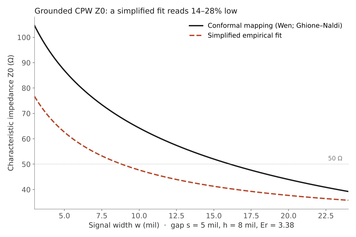
A designer trusting the fit would build a line near 70 Ω while aiming for 50 Ω. Use the published closed form, even when it needs an elliptic integral, and treat any formula without a citation as unverified.
10.2 Two valid models can disagree, so use one
Hammerstad–Jensen and IPC-2141 agree within −4% to +7% inside IPC-2141's range, but differ by up to 30% for wide traces (Figure 1). Independent comparisons rank Hammerstad–Jensen as the reference and advise caution with IPC-2141 outside its range [13]. When two tools in one flow use different models, the same geometry gets two impedances. Pick one model and use it throughout.
10.3 The constants in a rule of thumb matter
Rules of thumb are often re-derived with new constants. Two versions of the same √f/w conductor-loss law, both plausible at a glance, gave 0.188 dB/in (Bogatin's constant [7]) and 0.082 dB/in for an 8 mil, 76 Ω microstrip at 10 GHz. The second is 56% lower. Keep the published constant, or derive it from the copper's surface resistance.
10.4 Roughness depends on frequency
A fixed roughness multiplier is simple but wrong in trend. For 1 µm rms roughness a constant factor of 1.22 matches Hammerstad's correction at 1 GHz (1.20) but falls well short at 10 GHz (1.81) [1]. Since roughness loss grows as the skin depth shrinks, a frequency-independent factor understates loss exactly where high-speed links operate.
10.5 Nyquist is half the symbol rate, not the bit rate
For NRZ the bit rate and symbol rate are equal, so fN = bit rate / 2 is correct. PAM4 carries two bits per symbol, so its Nyquist frequency is bit rate / 4. Using bit rate / 2 for PAM4 places the evaluation point at twice the true frequency, where loss is much higher and the budget check meaningless.
10.6 Some parts have no useful formula
Connectors, packages and other three-dimensional transitions have no general analytical model; their behaviour depends on construction details no formula captures. A placeholder curve is acceptable while sketching, but it should be replaced with the vendor's measured or simulated S-parameters before any decision rests on it.
11. Validity at a glance
| Formula | Source | Stated validity |
|---|---|---|
| Microstrip Z0 and εeff | Hammerstad [3], Hammerstad–Jensen [1], Wheeler [2] | About 1% (1975); 0.01–0.03% (1980) |
| Microstrip Z0 | IPC-2141 [4], Kaupp [6] | 0.1 < W/H < 2.0 |
| Stripline Z0 | Cohn [5], IPC-2141 [4] | W/(b − T) < 0.35 |
| Grounded CPW Z0 and εeff | Wen [11], Ghione–Naldi [12] | Quasi-static, thin conductors |
| Dielectric loss | Bogatin [7] | Quasi-TEM lines |
| Conductor loss | Bogatin [7] | Skin-effect regime |
| Roughness factor | Hammerstad–Jensen [1], Huray [14] | Saturates at 2 (Hammerstad) |
| Er and Df versus frequency | Djordjevic–Sarkar [15] | Wideband Debye behaviour |
| Via L and C | Johnson–Graham [8] | Coarse estimate |
| Wire bond L | Rosa [18], Grover [19] | Wire much longer than its radius |
| Γ, RL, VSWR, ABCD | Pozar [9] | Exact |
| Crosstalk and eye | Johnson–Graham [8], Hall–Heck [20] | First order |
12. Conclusion
Analytical formulas remain the fastest way to reason about interconnects, and the standard ones are accurate to a few percent inside their ranges. Their failures come less from the physics than from how they are used: an uncited fit, two models mixed in one flow, a re-derived constant, a frequency-independent correction, a mis-stated Nyquist frequency or a formula asked to model a part it cannot.
We recommend citing a source for every formula a design depends on, staying inside its stated range, and checking any result that decides a design against a field solver or a measurement.
References
- E. Hammerstad and Ø. Jensen, "Accurate models for microstrip computer-aided design," IEEE MTT-S Int. Microwave Symp. Digest, Washington, DC, May 1980, pp. 407–409, doi:10.1109/MWSYM.1980.1124303.
- H. A. Wheeler, "Transmission-line properties of a strip on a dielectric sheet on a plane," IEEE Trans. Microw. Theory Techn., vol. 25, no. 8, pp. 631–647, Aug. 1977.
- E. O. Hammerstad, "Equations for microstrip circuit design," Proc. 5th European Microwave Conf., Hamburg, Sep. 1975, pp. 268–272.
- IPC-2141A, Design Guide for High-Speed Controlled Impedance Circuit Boards, IPC, Mar. 2004.
- S. B. Cohn, "Characteristic impedance of the shielded-strip transmission line," IRE Trans. Microw. Theory Techn., vol. 2, no. 2, pp. 52–57, Jul. 1954.
- H. R. Kaupp, "Characteristics of microstrip transmission lines," IEEE Trans. Electron. Comput., vol. EC-16, no. 2, pp. 185–193, Apr. 1967.
- E. Bogatin, Signal and Power Integrity — Simplified, 3rd ed. Prentice Hall, 2018.
- H. Johnson and M. Graham, High-Speed Digital Design: A Handbook of Black Magic. Prentice Hall, 1993.
- D. M. Pozar, Microwave Engineering, 4th ed. Wiley, 2012.
- B. C. Wadell, Transmission Line Design Handbook. Artech House, 1991.
- C. P. Wen, "Coplanar waveguide: A surface strip transmission line suitable for nonreciprocal gyromagnetic device applications," IEEE Trans. Microw. Theory Techn., vol. 17, no. 12, pp. 1087–1090, Dec. 1969.
- G. Ghione and C. Naldi, "Parameters of coplanar waveguides with lower ground plane," Electron. Lett., vol. 19, no. 18, pp. 734–735, Sep. 1983.
- F4INX, "Microstrip formulas comparison," f4inx.github.io/posts/microstrip-formulas-comparison.html.
- P. G. Huray et al., "Impact of copper surface texture on loss: A model that works," DesignCon, 2010.
- A. R. Djordjevic, R. M. Biljic, V. D. Likar-Smiljanic and T. K. Sarkar, "Wideband frequency-domain characterization of FR-4 and time-domain causality," IEEE Trans. Electromagn. Compat., vol. 43, no. 4, pp. 662–667, Nov. 2001.
- H. Johnson, "Via capacitance," High-Speed Digital Design newsletter, vol. 5, no. 9, sigcon.com/Pubs/news/5_9.htm.
- SI-LIST, "Approximations for partial self inductance," discussion with H. Johnson and E. Bogatin, qsl.net/wb6tpu/si-list/0117.html.
- E. B. Rosa, "The self and mutual inductances of linear conductors," Bulletin of the Bureau of Standards, vol. 4, no. 2, pp. 301–344, 1908.
- F. W. Grover, Inductance Calculations. Van Nostrand, 1946; Dover reprint, 2004.
- S. H. Hall and H. L. Heck, Advanced Signal Integrity for High-Speed Digital Designs. Wiley, 2009.
- IEEE Std 287-2007, IEEE Standard for Precision Coaxial Connectors (DC to 110 GHz).