How Much Data Is Enough? Part B: Predicting Where the Response Curves
Part A found where more data were needed after the fact, by adding points until the result stopped moving. Part B argues that the place can be predicted before solving. The guide is not the slope but the curve: a response curves where the design was tuned, at the 50 Ω match, and at frequencies set by its lengths, the ripples and the via-stub notch. Extra runs and finer frequency steps go there and nowhere else; tolerance then sets how many.
Introduction
Every interpolation assumes a shape between its points, and straight lines assume none. Part A showed that the error this leaves is set by curvature, |IL″|·h²/8, and that nothing in the data warns when it is large. Its remedy was to add points and watch.
That remedy is safe but blind: it spends runs everywhere to find the few places that need them. This note asks whether those places can be known in advance. We argue they can, from two things known before any solve: what the design was tuned to, and the lengths of its structures.
The argument has three steps. The slope is not the guide. The curve can be found from design and geometry, across both the inputs and frequency. Tolerance, last, sets how much extra data the curve needs. An experiment on a closed-form microstrip model tests each step.
Step 1: The slope is not the guide
It is natural to sample the most sensitive inputs most densely. But a steep response that is straight is captured exactly by two points; a flat response that bends is not. Loss tangent in Part A is the first case: a clear, steady effect that is linear to the last reported digit. Raw IL against substrate height is the second: almost no slope at nominal, yet the largest interpolation gap in the study.
The reason is an optimum. At any minimum the first-order term vanishes, and only curvature remains:
So the hardest place to sample is often where the response looks least sensitive.
Step 2a: Finding the curve across inputs
Why a tuned input curves
For insertion loss the optimum comes from the match. Reflected power is |Γ|² of incident power, and for small changes Γ grows in proportion to the impedance error [4]:
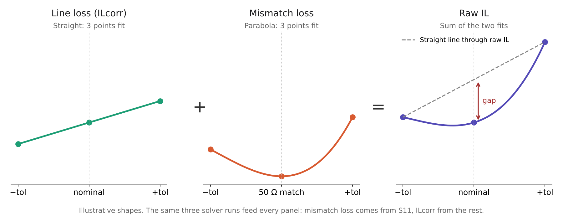
Any input the design was tuned on to reach 50 Ω, here substrate height, trace width and εr, therefore puts a bowl into raw IL at nominal. Inputs that do not move the impedance, such as loss tangent, do not. Removing reflections removes the bowl, which is why ILcorr stays nearly straight.
Experiment
We used a closed-form model as a stand-in solver: a lossy microstrip line between ports, with Hammerstad–Jensen impedance [3], skin-effect and dielectric loss, and an ABCD-matrix S-parameter calculation [4]. The baseline has a 127 µm substrate, εr = 3.66, 35 µm copper and tan δ = 0.004, with the width tuned to 50 Ω (276.5 µm). Lines of 0.5 mm and 10 mm were solved at 10, 20 and 40 GHz.
The predictions were written to a file first, using only how strongly each input moves the impedance. Each input was then stepped ±20% and solved at three points and on an 81-point sweep. As a control, the ports were changed to 40 Ω so that nominal was no longer the match.
| Prediction | Result |
|---|---|
| Inputs that move impedance (height, width, εr) gain extra curvature in raw IL | Confirmed: raw-IL gaps of 2–25% against ILcorr under 0.7% (0.5 mm line) |
| Inputs that barely move impedance (thickness, tan δ) do not | Confirmed: raw and ILcorr gaps both near 0% |
| Extra curvature ranks height, then width, then εr | Confirmed at all three frequencies and both lengths |
| The mismatch part has its minimum exactly at nominal | Confirmed: 0.0% offset for every impedance-moving input |
| With 40 Ω ports the minimum moves away | Confirmed: it moves to the edge of the ±20% range |
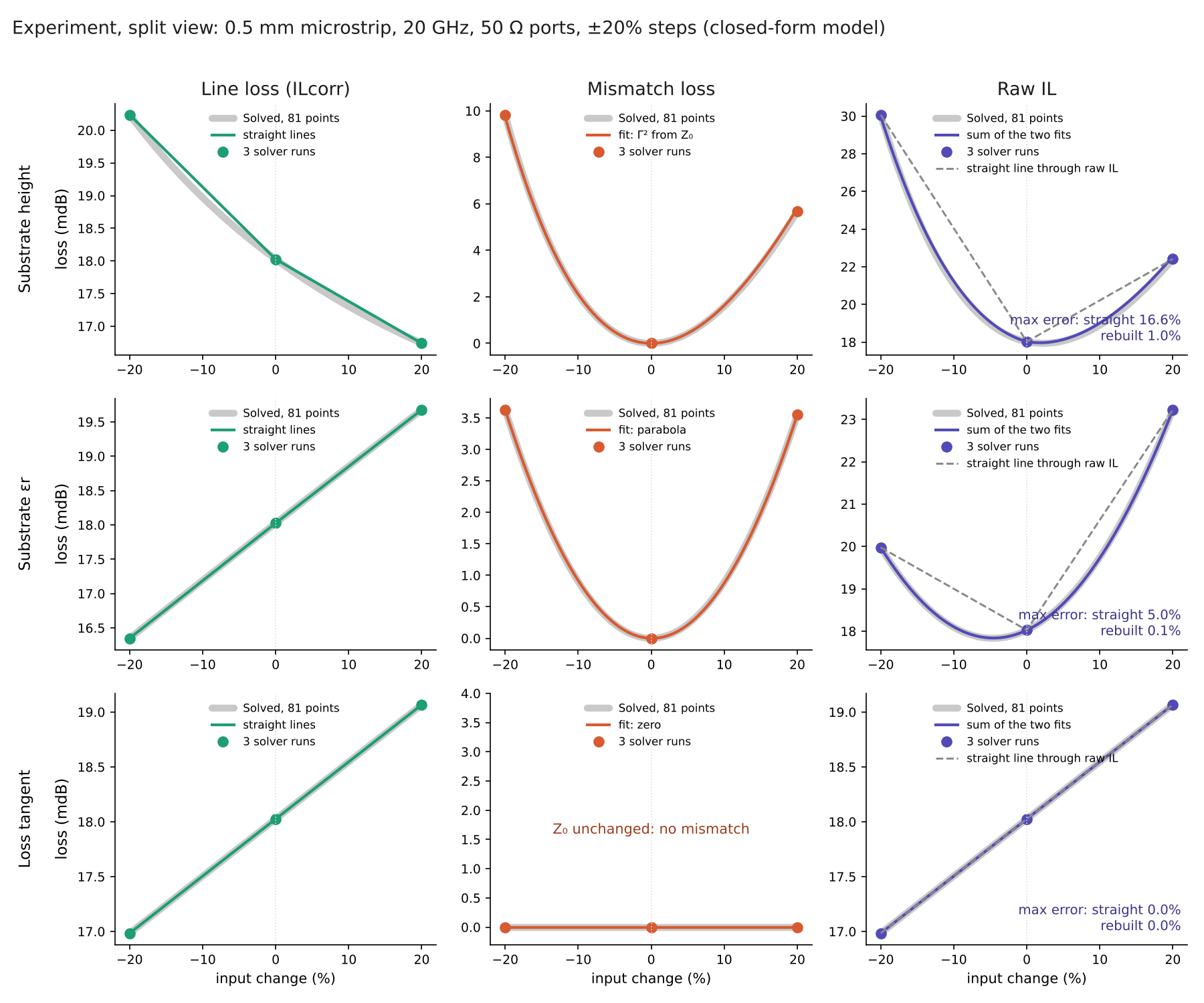
Read through the split of raw IL into line loss and mismatch loss, the same three runs show where the curve sits. Joining ILcorr with straight lines and fitting mismatch loss with a curve, then adding the two, recovers raw IL far better than straight lines through raw IL itself.
| Input | 10 GHz: straight / rebuilt (%) | 20 GHz: straight / rebuilt (%) | 40 GHz: straight / rebuilt (%) |
|---|---|---|---|
| Substrate height | 7.2 / 1.0 | 16.6 / 1.0 | 35.6 / 1.4 |
| Trace width | 4.7 / 0.7 | 10.8 / 0.8 | 23.4 / 1.5 |
| Substrate εr | 2.0 / 0.03 | 5.0 / 0.1 | 11.6 / 0.6 |
| Loss tangent | 0.0 / 0.0 | 0.0 / 0.0 | 0.0 / 0.0 |
Values are the largest error across ±20% as a percentage of baseline IL.
Step 2b: Finding the curve across frequency
Against frequency the curves come from lengths rather than from tuning, and they are just as predictable.
Ripple from line reflections
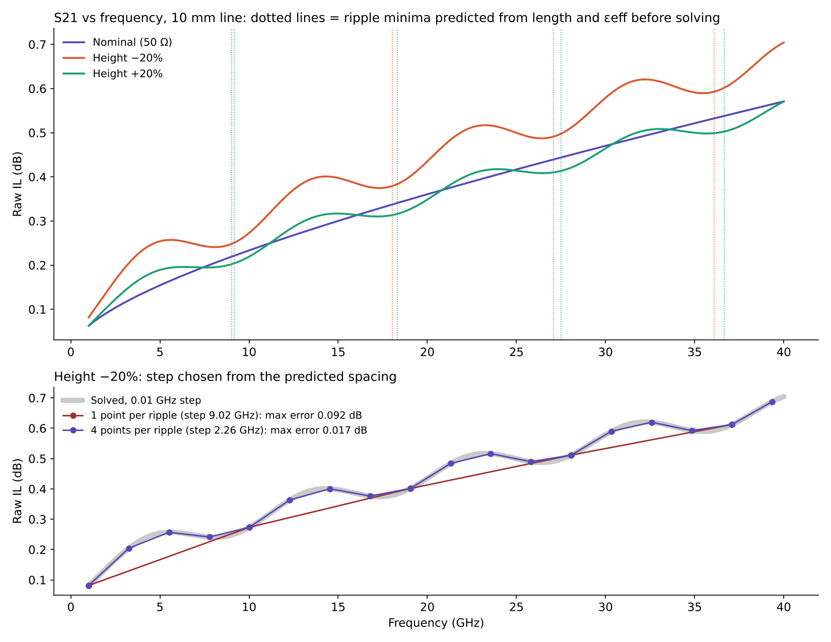
Reflections between the two ends of a mismatched line make S21 ripple at a regular spacing set by its electrical length:
For the 10 mm line this predicts a ripple every 9.02 GHz at −20% height and 9.16 GHz at +20%, and the solve put the reflection minima exactly there. The nominal 50 Ω line has no ripple at all, because it has nothing to reflect. A periodic ripple needs three to six points per period everywhere: one point per ripple slid through every ripple (0.092 dB error), four per ripple followed them (0.017 dB). For the 0.5 mm line the spacing is about 180 GHz, so a 0.1 GHz step is far finer than it needs.
A via-stub notch
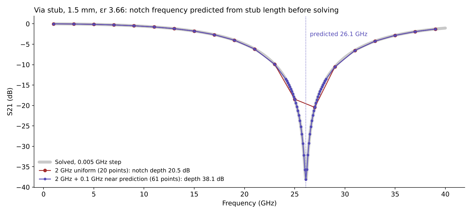
A through-hole via leaves an open stub that resonates where it is a quarter wavelength long:
For a 1.5 mm stub this predicts 26.1 GHz, and the solve put the notch at 26.11 GHz. The notch is narrow, about 0.2 GHz near its bottom, so a coarse uniform step jumps over it: 2 GHz everywhere (20 points) reported a 20.5 dB notch that is really 38 dB. A step of 0.1 GHz everywhere (391 points) caught it. So did 2 GHz everywhere plus 0.1 GHz within ±2 GHz of the prediction, with 61 points.
What the prediction cannot tell
Design and geometry predict where the response curves. They do not predict how much.
- Raw IL is not flat at nominal; only its mismatch part is. Line loss tilts the bowl, so raw IL's lowest point sits slightly off nominal.
- The exact shape can be wrong. A mismatch model built from the impedance alone fits height and width but fails for εr, which also changes the electrical length (3.7% error against 0.1% for a plain parabola). Because that model has one free number, the three runs themselves reveal the miss.
- The depth and width of a notch, and the size of a ripple, depend on loss and coupling and must come from the solve. Pad and anti-pad capacitance also pull a real via notch somewhat below c / (4·L·√εr).
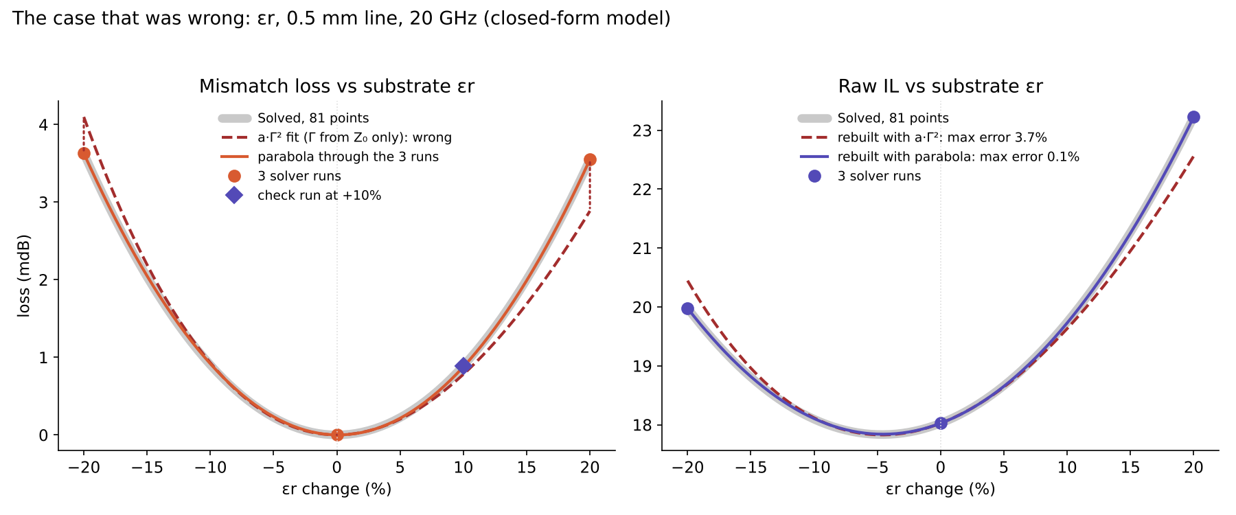
So the prediction decides where to look; Part A's check, adding a point and seeing whether the result moves, still decides when to stop.
Step 3: Tolerance sets how much
Tolerance design treats the scatter of built parts as part of the design problem [1, 2]. For sampling, its use is narrow but decisive: once the curve is located, tolerance sets how wide a region around it matters, and the gap grows with the square of that width.
Across inputs, only the real tolerance range needs to be accurate. Scaling Part A's measured gaps at 40 GHz:
| At 40 GHz | ±20% (Part A) | ±10% | ±5% |
|---|---|---|---|
| Raw IL, substrate height: gap / points | 6.5% / 7 | 1.6% / 4 | 0.4% / 3 |
| Raw IL, substrate εr: gap / points | 3.1% / 5 | 0.8% / 3 | 0.2% / 3 |
| ILcorr, any input: gap / points | ≤0.6% / 3 | ≤0.15% / 3 | ≤0.04% / 3 |
Points are for a gap under 1% of baseline IL, spread evenly across the range, with three as the minimum so that curvature can be detected at all. When the tolerance is not yet known, plan for ±20% and cut back once the fabricator confirms.
Across frequency, tolerance sets the width of the fine-step band, because built parts do not share one notch frequency:
A ±10% backdrill depth and ±2% εr move the 26 GHz notch by about ±11%, or ±2.9 GHz, which is the band the fine step must cover.
Summary
| Step | Across inputs | Across frequency | Data |
|---|---|---|---|
| 1. The slope is not the guide | A steep, straight response needs three runs | A smooth slope needs only a coarse step | No extra data for steepness alone |
| 2. Find the curve | At the 50 Ω match, for inputs the design was tuned on | At ripples, c / (2·L·√εeff), and at stub notches, c / (4·L·√εr) | Extra runs for tuned inputs; 3–6 points per ripple; fine steps around a notch |
| 3. Tolerance sets how much | Sample over the real tolerance, not the test range | Fine band wide enough for the notch to move | Points from the 1% rule; band from Δf / f |
| Check | Add a run and see whether the result moves | Tighten the step until the notch depth stops moving | Confirms the count |
The closed-form model has no launch structure, radiation, dispersion or roughness, so it confirms the mechanism rather than any full-wave number. The same comparison on EM data is the next test.
References
- R. Spence and R. S. Soin, Tolerance Design of Electronic Circuits. Addison-Wesley, 1988; reissued by Imperial College Press, 1997.
- A. Ilumoka and R. Spence, "Parameter tolerance design for electrical circuits," Quality and Reliability Engineering International, vol. 4, no. 2, 1988, doi:10.1002/qre.4680040203.
- E. Hammerstad and Ø. Jensen, "Accurate models for microstrip computer-aided design," IEEE MTT-S Int. Microwave Symp. Digest, 1980, pp. 407–409, doi:10.1109/MWSYM.1980.1124303.
- D. M. Pozar, Microwave Engineering, 4th ed. Wiley, 2012.