Why Simulation vs Measurement Correlation Remains a Key Challenge for SI Teams
Simulation and measurement disagree on almost every high-speed board. The disagreement is rarely a solver bug. It is the sum of small differences in material data, copper, ports and fixtures that nobody wrote down, spread across people, tools and files.
A familiar story
A channel is simulated. The eye opens, the loss sits inside budget, and the design goes to fab. Weeks later the first boards come back and someone takes a VNA sweep.
The measured insertion loss is steeper than the model. The return loss has ripples that were never in the simulation. And the same question comes up every time: is the model wrong, is the board wrong, or is the measurement wrong?
Published comparisons put routine gaps at 2 to 8 percent on insertion loss. That sounds small. But spread over a long route at 16 GHz, a few tenths of a dB per inch can decide whether a PCIe or Ethernet link passes. We looked at where those gaps come from in detail in Simulation–Measurement Correlation in High-Frequency Planar Structures. This post is about why closing them stays hard in practice.
Five reasons the gap persists
1. Material data is a datasheet guess
Laminate Er and Df are quoted at one or two frequencies, for one glass style and resin content. The pressed prepreg in your stackup has a different resin content, so its Er is lower than the core's. Df also rises with frequency.
If the model uses a 1 GHz value at 8 GHz, it is optimistic before any other error is added. Choosing the right material for the frequency is covered in The Role of Data Rate in Laminates Thermal Limits and Cost Tradeoffs.
2. Copper is never smooth
Conductor loss grows with frequency as current crowds into the skin of the copper, and on a real board that skin is rough. Standard, reverse-treated and very-low-profile foils can differ by tens of percent in conductor loss. A model with smooth copper will undershoot a long line every time.
3. Ports and fixtures change what is measured
This is the most underestimated source. A solver's wave port is a perfect, de-embedded launch. A real measurement goes through a connector, a launch pad or a probe, each with its own reflection.
FlowSimLab's dataset table shows how big this is. For the same 52.1 Ω microstrip, return loss at 5 GHz is about −35 dB with a de-embedded wave port and about −25 dB with a GSG probe, while insertion loss barely moves. Compare a de-embedded model with a raw measurement and S11 will never agree.
4. Nobody records the setup
Surface finish, solder mask, port type, de-embedding and instrument settings all change the result. Yet they usually live in a lab notebook, an email, or nowhere. Six months later, no one can say whether the 2 dB gap was the board or the cable.
5. Results live in different tools
The stackup sits in one file, the field solver in another, the VNA data on a lab PC and the budget in a spreadsheet. Correlation needs all four side by side. Gathering them is enough work that it often gets skipped.
How FlowSimLab approaches correlation
FlowSimLab is built on one idea: correlation starts when the trace is defined, not after the board comes back.
In the Single-ended trace step you enter topology, stackup, geometry, copper and termination, and the impedance updates as you type.
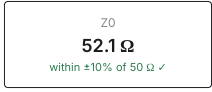
Underneath, FlowSimLab pulls the closest simulated datasets for the same geometry and tags each one with surface finish, solder mask, port and copper foil. That is the correlation checklist made visible. Before any board is built, you can see how much a port or a foil changes the answer, and decide what your measurement has to match.
Pick a dataset and its insertion loss is plotted against the model.
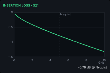
When boards come back, the same card takes the measurement. You upload a touchstone file or pick an existing one, and it is stored with its build and setup details: surface finish, mask, fixture, de-embedding, instrument and date. The context that usually gets lost now travels with the data, and the plots show model and measurement together, along with the band that contains the whole measurement.
A simple correlation routine
- Use Er and Df at your Nyquist frequency, and estimate pressed prepreg separately.
- Match the copper foil to what the fab actually uses.
- Match the model's port to the board's launch, or de-embed the measurement.
- Record finish, mask, fixture and instrument with every measurement.
- Compare insertion loss first; read return loss second, since launches dominate it.
- Explain the remaining gap one cause at a time, and keep the explanation with the data.
If the S-parameter plots themselves are unfamiliar, start with How to Interpret S21 S11 and Eye Diagrams for Quick Assessments.
The bottom line
Correlation stays hard because the gap is the sum of many small, undocumented choices. Solvers are rarely the weak link. Keeping the assumptions visible and attached to the results is what closes the gap, and that is what FlowSimLab's trace step and measurement records are built to do.
Want to see it on your own stackup? Talk to our team or sign up for access.