Step by Step Channel Setup Using FlowSimLab DSS for High Speed Designs
FlowSimLab breaks channel setup into a short sequence of steps, each one feeding the next: material, channel, trace, group, layers, bumps, parts and standards. Then the DSS lets you explore any trace in depth, with S-parameters, TDR and eye diagrams. This guide walks through every step, with one example carried all the way through.
Before you start
Everything in this guide happens in your browser. You need an account, and you will spend most of your time on the dashboard, which lays out the setup as numbered cards. Each card opens into a panel where you enter values and see results, and each one passes what it learned to the cards after it.
A few things are useful to have to hand:
- The interfaces on your board and their data rates.
- The longest route for each high-speed link, even as a rough estimate.
- Your target layer count and board thickness.
- The laminates your fab can offer, if you already know them.
You do not need all of this to begin. FlowSimLab starts from sensible defaults, and every value can be changed later. The point is to replace those defaults with your real numbers as you go.
Projects and units
Work is organised into projects, listed in the panel on the left of the dashboard. Each project keeps its own material, channels, trace types, groups, stackup and ball map, so you can try a variant without touching the original. Project settings also hold your preferred units for geometry and length, so everything reads in mil and inches, or in µm and mm, consistently across every step.
Our example throughout is a PCIe Gen4 link from a host processor through a CEM connector to an add-in card.
Step 1: Material selection
The first step picks the laminate. It comes first because almost every later number, from loss per inch to impedance, depends on it.
Enter the requirements
The top of the panel asks for what the signals need:
- Fastest rate and signalling (NRZ or PAM4).
- Longest route and its loss budget.
- Layer count.
- Lead-free assembly, yes or no.
- Operating environment.
From these, FlowSimLab works out the Nyquist frequency and the loss per inch your laminate has to meet.

Read the candidate table
Below the requirements is a table of candidate laminates, recalculated at your Nyquist. For each one you see Er, Df, loss per inch, route loss, Tg and Td, z-CTE, core thickness, cost relative to FR4 and an overall fit. A thermal warning appears when a material's Tg, Td or z-CTE is not a good match for your layer count or lead-free assembly.
Quick filters narrow the list when the constraint is not loss: cheap, thin cores, low loss, RF-stable Er, high Tg, FR4 process or stocked at most fabs.
Compare two on the spider chart
Tick two materials and the property spider draws them side by side.
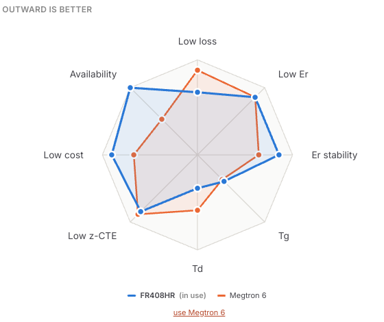
Each axis is a property where outward is better: low loss, low Er, Er stability, Tg, Td, low z-CTE, low cost and availability. It turns a wall of numbers into a picture of the tradeoff. Here Megtron 6 reaches further on loss, while FR408HR reaches further on cost and availability.
Choose copper and stackup approach
Two more choices finish the step. The copper foil (for example reverse-treated) scales the conductor loss. The stackup approach is either a single material for every layer, or a hybrid that uses the fast laminate only for the high-speed layers and a cheaper one elsewhere.
Finally, mark whether your fab has confirmed the values, pick a priority (cost, balanced or loss), and save the project material. For our PCIe Gen4 example, FR408HR is the choice.
For the reasoning behind these choices, see The Role of Data Rate in Laminates Thermal Limits and Cost Tradeoffs and A Practical Guide to Laminate Selection for PCIe and Ethernet Interfaces.
Step 2: Channel
The Channel step builds the loss budget for each link, from transmitter to receiver.
Choose the interface
Pick the interface from the list, for example PCIe Gen4. FlowSimLab fills in the data rate, signalling and a typical insertion-loss budget. You add a margin, the amount you want to hold back for tolerances and surprises; 3 dB is a common choice. A Custom interface lets you enter your own budget.
Add the parts
Next, list the parts in order. FlowSimLab supports packages, PCB routes, vias, connectors, cables and other parts. Fixed parts take a loss in dB at Nyquist. PCB routes take a length and use the project laminate's loss per inch. Vias take a count and a loss per via.

Click any part to see a drawing of it. Parts can be reordered, duplicated and removed, and a colour bar shows each part's share of the budget.
Read the result
The result panel compares the total with the budget.
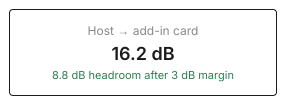
It also breaks the PCB loss into dielectric and conductor parts, and works out the longest total PCB length the budget allows, 20.75 inches in our example. That number is worth giving to whoever does the layout.
You can add as many channels as the board has, and duplicate a channel to try a variant. The method is explained further in How to Budget Loss and Impedance for Multi Layer PCB Stacks.
Step 3: Single-ended trace
This step defines trace types: the actual geometry each route will use.
Name it after the route
Start by picking a PCB route from step 2 as the trace type name. This link matters. It is how the Standards step later knows which trace geometry belongs to which route.
Set the geometry
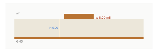
Choose microstrip or stripline, then enter the stackup (Er and dielectric height), the trace width and length, and the copper weight. The cross-section updates as you type.
Hit the impedance target
Set a target impedance and tolerance, and use Solve width to find the width that hits it. The results panel shows the impedance and whether it is inside tolerance.
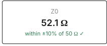
Alongside it you get effective Er, delay per inch, total propagation delay, loss at Nyquist split into dielectric and copper, and the reflection against your termination. A "line behaves as" field tells you whether the trace is long enough to act as a transmission line for your rise time, or short enough to be treated as a lumped connection.
Check the matching datasets
Below the inputs, FlowSimLab lists simulated datasets that match your geometry, each tagged with surface finish, solder mask, port type and copper foil. Click one to see its eye diagram, insertion loss and return loss.
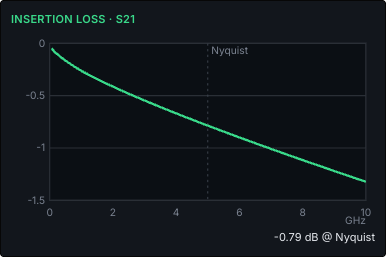
This is also where measurements live. You can upload a measured file or select an existing one, and it is stored with its build and setup details for later comparison. Why that matters is covered in Why Simulation vs Measurement Correlation Remains a Key Challenge for SI Teams.
Save the trace type, then repeat for each route that needs one.
Step 4: Group
The Group step collects nets into groups that share routing rules.
Create a group
Give the group a name, such as "DDR4 byte 0", and choose a kind. Each kind comes with sensible starting rules:
- Bus: 50 mil match tolerance, 6 inch maximum length, 2 vias, 3W spacing, GND reference.
- Clock: 25 mil match, 4 inches, 2 vias, 5W spacing, GND reference.
- Strobe + data: 10 mil match, 3 inches, 2 vias, 3W spacing, GND reference.
- General: 500 mil match, 10 inches, 4 vias, 2W spacing, either plane.
Add nets and tune the rules
Add nets to the group. You can type a range like "DIG 1-8" instead of every name. Each net is linked to one of your trace types, and the routing rules can be adjusted: match tolerance, maximum length, maximum vias, spacing, reference plane, and whether crosstalk should be checked.
The checks panel then reports length and delay skew, crosstalk and any rule that is broken. Nets that are not yet in any group are listed so nothing gets forgotten.
Step 5: Layers
The Layers step builds the stackup and places each group on a layer.
Build the stackup
Choose a layer count and a target board thickness. FlowSimLab starts from a standard stackup for that count, which you can edit layer by layer: signal, ground, power or mixed, with copper weight, and the dielectric between each pair as core or prepreg with its thickness.
Check it
The checks panel confirms the board thickness against your target.
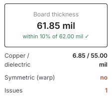
It also reports copper and dielectric totals, whether the stackup is symmetric (asymmetric boards bow and twist), and any issues. Each signal layer is shown with the planes it references and whether it behaves as microstrip or stripline.
Assign groups to layers
Put each group on a layer. The 3D view then shows the vias from the top of the board down to each layer, with the leftover stub labelled.
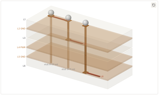
Long stubs resonate near a quarter wavelength, so this view is a quick way to spot a layer choice that will cause trouble at high data rates. Our example's 61.51 mil and 37.11 mil stubs resonate near 25 GHz and 42 GHz, which is fine for PCIe Gen4.
Step 6: Bumps
The Bumps step assigns nets to the package's bumps or balls and checks the path down to each layer.
Set the grid and pattern
Enter rows, columns and pitch (39.37 mil is a 1 mm pitch), then pick a signal-to-ground pattern such as S:G 2:1.
Assign nets
Use Auto-assign to place your groups using the pattern, or paint by hand with the brush: nets, GND, PWR or erase. You can filter the map by group or search for nets.
Follow the path down
The summary reports signal, ground and power counts, the actual signal-to-ground ratio, nets placed, free bumps and the worst via stub. The 3D view switches between bump-to-bump and bump-to-layer, with through, back-drilled, blind or stacked micro-via styles.
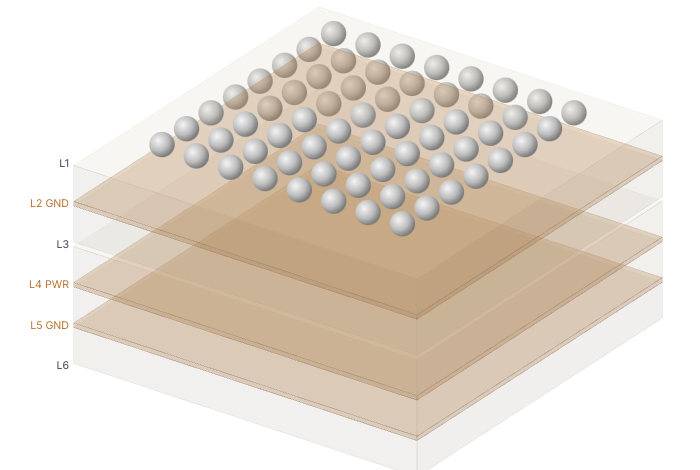
More on this step in Chip Packaging Transitions from Package to Board Explained.
Step 7: Component library
Between bumps and standards sits the Component Library. It is where you find realistic values for the parts in your channel: vias, microstrip, grounded CPW, stripline, wire bonds and coaxial connectors.
Each component has a set of variables you can constrain, and a large table of datasets that updates as you filter. The best match is shown at the top, ranked by the metric you choose.
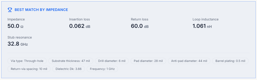
Use the results to replace the default via and connector losses in your channel with values for the parts you will actually use. See Choosing Vias and Connectors for High Speed Data Paths for what to look for.
Step 8: Standards
The last dashboard step compares everything with the interface standards.
For each channel, FlowSimLab runs four checks: insertion loss from step 2, impedance from the trace types in step 3, laminate loss from step 1 and return path from the stackup in step 5. Each one shows Pass, Check or Fail with a value and a reason.

In our example, everything passes except impedance, which is flagged until the host and add-in routes are linked to trace types. That is a reminder to go back to step 3, not a problem with the design. A full guide to these checks is in How to Use Standards Checks to Accelerate PCB Sign Off.
Exploring a trace in the DSS
The dashboard steps set the channel up. The DSS, at /software/dss, is where you explore a single trace in depth. It has two modes, Workbench and Flow, switched with a toggle at the top.
Workbench mode
The Workbench is a free-form panel. Stackup, geometry and source settings are on the left, a layout or scope view in the middle, and results on the right: impedance, propagation delay, insertion loss and reflection. It is the quickest way to answer "what if I make this trace 1 mil wider?"
Flow mode
Flow mode is a guided, nine-step sequence that teaches and builds at the same time. Each step opens with a short explanation, then asks for input or shows a result. A data-source switch at the top lets you work from calculation, your own custom data, a part, or a target output.
Here is what each step does.
Flow step 1: Stackup
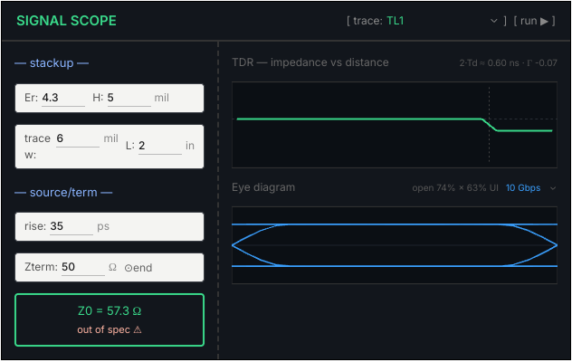
Enter Er, dielectric height and copper thickness. The Signal Scope beside it shows the impedance, a TDR trace and an eye diagram, all updating live.
Flow step 2: Simulate S-parameters
Run a frequency-domain simulation. FlowSimLab computes S21 (insertion loss) and S11 (return loss) from the line's ABCD matrix and sweeps up to the signal's knee frequency, 0.35 divided by the rise time.
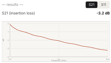
Toggle between S21 and S11 to read both. If you are new to these plots, read How to Interpret S21 S11 and Eye Diagrams for Quick Assessments first.
Flow step 3: Compare configurations
Set up variants side by side, each with its own width and termination, and compare their impedance and TDR.
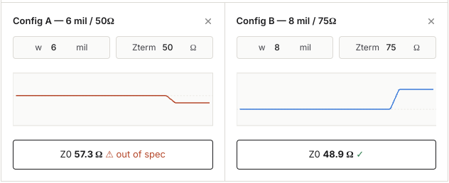
It is the fastest way to see which combination lands in spec.
Flow step 4: Signal path and length matching
For multi-drop nets such as a DDR fly-by bus, every branch has to arrive at the same time. Draw the topology, set each segment length and a match tolerance, and any branch whose skew exceeds it is flagged.
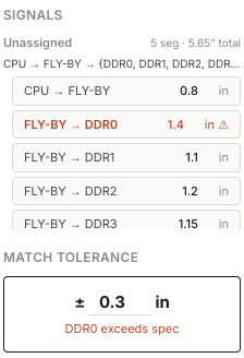
Flow step 5: Board layout
Place the net on the board and inspect coupling. The left panel switches between nets, layers and diff pairs, with common high-speed interfaces preloaded. The results show impedance, insertion loss and worst-case near-end crosstalk.
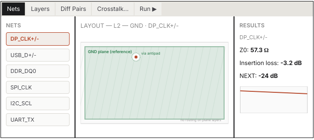
Flow steps 6 and 7: Trace geometry, source and termination
Set the routed width and length, then the driver rise time, data rate and termination. Width trades directly against impedance; length drives delay and loss. Rise time decides how high in frequency the simulation needs to go.
Flow step 8: Your trace types
Review the trace types you have built. Add the current one, or switch between saved types using the dropdown in the instrument.
Flow step 9: Save
Save your trace types to complete the first phase. They become available to the rest of the project.
Putting it all together
Here is our PCIe Gen4 example, end to end:
- Material: FR408HR, chosen over Megtron 6 on the spider chart for cost and availability.
- Channel: 16.2 dB against a 28 dB budget, 8.8 dB headroom, 20.75 inch maximum PCB length.
- Trace: an 8 mil microstrip at 52.1 Ω, inside ±10%.
- Group: the PCIe pair grouped with its own rules.
- Layers: a 6 layer, 61.85 mil board with every signal layer next to a plane.
- Bumps: the PCIe signals placed with neighbouring grounds.
- Library: via and connector losses replaced with real part values.
- Standards: zero fails, with the remaining checks resolved or explained.
The DSS was used along the way to compare widths and terminations and to read the eye before committing.
Tips for a smooth setup
- Work through the steps in order the first time. Later, jump to whichever step needs changing; the others update.
- Name trace types after the routes they belong to. It is the one link the Standards step relies on.
- Keep the Standards step open while you work. It is the fastest feedback loop in the tool.
- Use projects for variants instead of overwriting your baseline.
- Mark laminate values as confirmed only once your fab has confirmed them.
- Treat every number as a first-order estimate, and confirm critical structures with a full-wave solve and measurement.
For a printable version of the sequence, use From Requirements to Sign Off: A Practical High Speed Channel Checklist. To set this up on your own design, sign up or talk to our team.